ESCO凸轮走心机节拍计算详解：基于Ø2.5mm轴类零件的完整工艺分析

ESCO走心机以其精密的节拍控制和高效的生产能力而闻名于世。本文将以直径2.5mm轴类零件为例，深入解析ESCO凸轮走心机节拍计算的完整流程，揭示其核心技术原理。二手ESCO机台及ESCO型全新数控Y2-CNC机台垂询电话：139 1634 2943

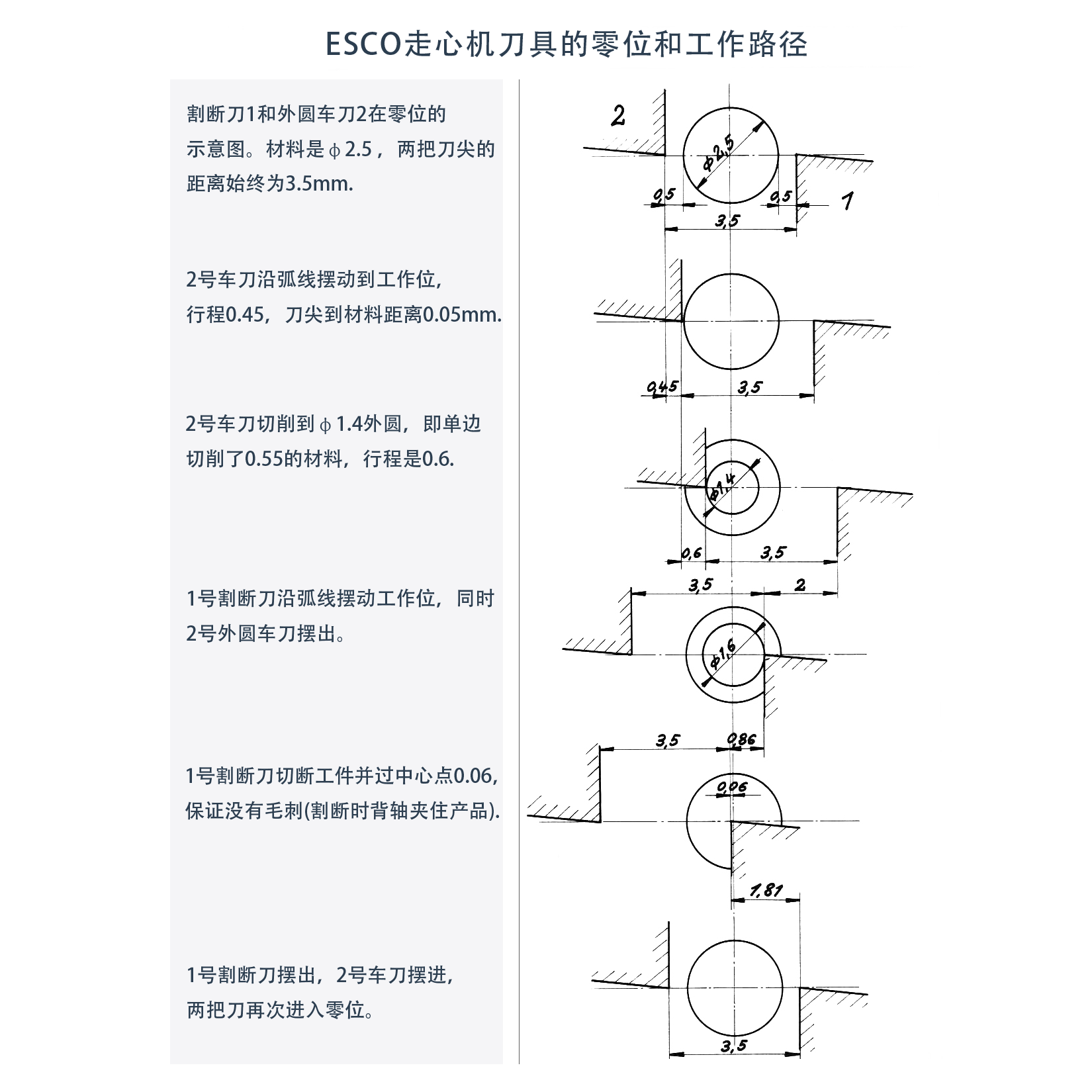
图1：ESCO走心机刀具布局和工作路径示意图 - 展示了刀具零位设定与多工序协调作业流程

一、工序分解与参数设定

1. 加工工序序列

ESCO走心机的加工过程严格按照预设的工序序列执行，每个工序都有明确的刀具动作和关联动作：

工序	刀具动作	关联动作
a	刀具2切入：Ø3.5 → Ø2.6mm	刀具1空程退出
b	刀具2倒圆角：Ø2.6 → Ø1.4mm	刀具1退至Ø5.6mm
c	刀具2暂停切削	-
d	刀具1切入：Ø5.6 → Ø1.6mm	刀具2退至Ø5.4mm
e	刀具1切断（超中心0.06mm）并修尖	-
f	刀具1暂停	-
g	刀具1退回零位（Ø3.5mm）	-
h	材料进给17mm（工件长16mm+切断刀宽1mm）	-
i	反向夹头闭合（进给结束时）	-
j	反向夹头开启（切断后）	-

关键规则：无纵向车削时，夹头全程闭合直至切断完成

2. 工序协调原理

ESCO凸轮系统的核心优势在于多刀具的精确协调：

刀具1负责切断和精加工
刀具2负责粗加工和倒角
反向夹头确保工件稳定夹持
材料进给系统实现连续生产

二、工作行程与进给量计算

1. 工作行程量化（单位：0.01mm）

精确的工作行程计算是节拍控制的基础：

工序	工作行程	计算依据
b（倒圆角）	60	Ø2.6→Ø1.4mm = 径向切深0.6mm
e（切断）	86	切断深度0.86mm

2. 刀具每转进给量（单位：0.01mm/rev）

进给量的设定直接影响加工质量和效率：

工序	进给量	参考标准
b（倒圆角）	1.15	精车标准值
e（切断）	0.80	切断标准值

3. 刀具转数计算

计算公式：

转数 = 工作行程 / 进给量

具体计算：

倒圆角：60 / 1.15 ≈ 52.17 → 52转
切断：86 / 0.80 = 107.5 → 108转

有效加工总转数 = 52 + 108 = 130转

三、非生产时间转换（凸轮度数）

1. 非生产动作时间表

非生产时间的精确控制是提高效率的关键：

工序	动作说明	凸轮度数
a	刀具2切入空程（0.45mm）	16°
c	刀具2暂停	2°
d	刀具1切入空程（2mm）	17°
f	刀具1暂停	2°
g	刀具1退回（1.82mm）	18°
h	材料进给17mm	59°
总计		110°

计算依据：

空程每0.5mm ≈ 16-20°（查表页52）

进给17mm = 59°（查表页52）

2. 时间分配优化

非生产时间的合理分配确保了：

刀具切换的平稳性
材料进给的精确性
系统运行的稳定性

四、节拍核心计算

1. 时间平衡方程

ESCO凸轮走心机节拍计算的核心是时间平衡：

总凸轮周期(360°) = 有效加工时间 + 非生产时间 + 安全余量

2. 计算实际刀具转数需求

可用生产角度计算：

可用生产角度 = 360° - 110° = 250°

有效加工转数密度：

130转 / 250° = 0.52转/度

总刀具转数需求：

130 × (360° / 250°) = 187.2 → 188转

3. 产能匹配验证

挂轮表查找：

188转 → 32件/分钟

g系数修正（经验因子）：

类比页42类似工件形状，取g=1.4
理论转数 = 130 × 1.4 = 182转
实际188转满足要求

五、凸轮角度分配

1. 计算公式

工序凸轮角度分配公式：

工序凸轮角度 = (工序转数 × 360°) / 总刀具转数

2. 切断工序示例

切断工序（78转）计算：

(78 / 188) × 360° = 149.36° → 149°

3. 凸轮相位分布

0°→149°：切断修尖
149°→167°：刀具1暂停
167°→185°：刀具1退回
185°→244°：材料进给
...（其他工序按同理分配）

六、双锥耦合进给系统优势

1. 与传统夹头对比

指标	ESCO双滚轮系统	传统夹头系统
夹紧动作时间	0°（持续夹持）	需8-10°开合
材料回退时间	集成在切断周期内	额外15-20°
最小节拍限制	32件/分钟	≤25件/分钟

2. 双端细长工件特殊处理

面临的挑战：

需全程纵向车削 → 无空闲时间回退进给杆

解决方案：

采用40°短行程凸轮（替代标准65°）
移除可调限位块
凸轮角度计入生产节拍

3. 系统优势总结

高精度夹持：双锥设计确保工件同心度
连续进给：无需频繁开合夹头
节拍优化：减少非生产时间
质量稳定：±0.01mm的尺寸稳定性

七、关键公式总结

1. 有效转数密度

K = 有效加工总转数 / 可用生产角度

2. 总刀具转数

N总 = (有效加工总转数 × 360°) / (360° - θ非生产)

3. 工序角度分配

θ工序 = (N工序 × 360°) / N总

八、实际应用与调试要点

1. 精度要求

凸轮相位误差≤0.1°
尺寸稳定性±0.01mm
表面粗糙度Ra≤1.6μm

2. 调试验证

使用分度盘验证凸轮相位
测量实际切削力和振动
监控刀具磨损情况

3. 优化建议

根据材料特性调整进给量
优化刀具几何角度
定期校验凸轮精度

结语

ESCO走心机节拍计算体系通过凸轮角度-刀具转数的精确映射，实现了微细轴加工的高精度和高效率。这套计算方法不仅适用于Ø2.5mm轴类零件，更为其他规格产品的工艺设计提供了科学的理论基础。

在实际生产中，准确的节拍计算是实现自动化生产的前提，而ESCO系统的双锥耦合进给技术则为传统机械加工向现代精密制造的转型提供了宝贵的技术参考。

通过深入理解这些计算原理，工程技术人员可以更好地发挥ESCO走心机的技术优势，实现更高的生产效率和产品质量。

ESCO走心机节拍计算详解：基于Ø2.5mm轴类零件的完整工艺分析